Uncertainty in water body assessment
01 WISER improved the knowledge on the sources of uncertainty in ecological status classification
Key message
Knowing the main sources of uncertainty in WFD metrics informs the design of effective WFD monitoring programmes, assessment of ecological status and design of programmes of measures. The WISER project has improved our understanding of many of these sources of uncertainty.
Evidence
In the WISER project, an understanding of several potential sources of sampling uncertainty (spatial, sampling/sample processing) was built into the foreground sampling programme, aspects of temporal uncertainty could be investigated using the collated background datasets. However WISER uncertainty analysis was not able to address ALL potential sources of uncertainty in any individual BQE. Results from lake phytoplankton and macrophyte uncertainty analysis show that between-lake variation in metrics is greater than within-lake variation and between-analyst variation. Within-lake variation in phytoplankton metrics was small, and within-lake variation in macrophyte metrics was generally consistent and could be managed by sampling sufficient replicate transects. These results give confidence in the use of these BQEs for waterbody-level assessment of ecological status.
Implication
Understanding of the different sources of uncertainty and their relative magnitudes makes uncertainty manageable and is an essential part of the design of effective monitoring programmes. This includes standard protocols for sampling and laboratory processing, and it includes consistent staff training. The methodological requirements for a sampling programme for WFD status assessment may differ from those of more academic study. Current monitoring programmes may have replication where it is not needed, while they may be ignoring other more important aspects of uncertainty. Uncertainty exists in all freshwater biomonitoring, ideal BQEs which responds strongly to single stressors and can be measured with minimal uncertainty are rare or non-existent. Authorities should acknowledge uncertainty in reporting all water body assessments.
Further reading
Detailed descriptions of the data basis, analytical methods and results may be found in WISER Deliverable D3.1-3 ('Report on uncertainty in phytoplankton metrics') and D3.2-2 ('Report on uncertainty in macrophyte metrics').
02 Uncertainty may vary between different metrics calculated for the same BQE
Key message
Many different assemblage metrics (e.g. using various combinations of taxon tolerance values, richness, abundance, traits) can be calculated for a single BQE. The selection of candidate metrics for assessment should be informed by the residual sampling variance of individual metrics, as well as their indicator value for particular stressors. This variability can itself vary considerably among different metrics describing the same BQE.
Evidence
Some comparisons could be made between alternate metrics based directly on taxonomic composition (including morpho-types) and metrics based on bio-physical (e.g. macrophyte maximum colonisation depth) or biochemical measures (e.g. chlorophyll a concentration). Results were mixed. Improved taxonomic resolution reduces uncertainty of taxonomy-based metrics: Phytoplankton PTI metric (taxonomic) showed clearly lower uncertainty than SPI metric (based on phytoplankton size groups). Replicate sampling uncertainty for chlorophyll a was low.
Implication
In general, metrics with low sampling uncertainty relative to their stressor response should be used. Metric specification is likely to need to include specification of sampling and laboratory protocols. Status assessment can be made more precise if it combines taxonomic and biophysical/biochemical measurements which show low sampling uncertainty, but metrics with high sampling uncertainty should not be used or combined.
Further reading
Detailed descriptions of the data basis, analytical methods and results may be found in WISER Deliverable D3.1-3 ('Report on uncertainty in phytoplankton metrics') and D3.2-2 ('Report on uncertainty in macrophyte metrics').
03 The WISER Bioassessment Uncertainty Guidance Software (WISERBUGS) helps water managers quantify the sampling uncertainty and confidence of water body ecological status classification
Key message
The new WISER Bioassessment Uncertainty Guidance Software (WISERBUGS) provides a flexible general means of using sampling uncertainty simulations to assess confidence in estimates of Ecological Quality Ratios (EQRs) and derived WFD ecological status class for water bodies. Assessments may be based on single metrics or a combination of metrics including multi-metric indices (MMIs) and multi-metric rules and involving metrics from one or several Biological Quality Elements (BQEs) for any type of water body with appropriate data.
Evidence
Users must provide prior estimates of the relevant sampling uncertainty for each metric to be involved in their water body assessments, together with metric status class limits and the rules for combining metrics and maybe BQEs into an overall water body assessment. Options include worst-case (One-Out-All-Out), mean and median class rules and the use of weighted multi-metric indices. Several WISER deliverables provide examples of how to derive the relevant sampling uncertainty measures for input to WISERBUGS (see also Figure 1).
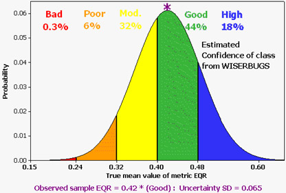 Figure 1
Implication
The WISERBUGS software can help agencies with monitoring responsibilities and catchment managers quantify the confidence associated with their estimates of water body WFD status class, as required by the WFD. It is especially useful for providing water body classifications and the confidence consequences for multi-metric and multi-BQE integrated assessments in both trial and operational use. It can be used for metric EQR-based status class assessments of any type of water body (rivers, lakes, transitional or coastal waters).
WISERBUGS can also be used just to test the effect of new status class limits and multi-metric rules on site/waterbody status assessments, without any uncertainty assessment (by setting all uncertainty components to zero).
Further reading
WISERBUGS is available for download in the software section (Windows version only). A documentation of the software and its applications is available as WISER Deliverable D6.1-3.
04 Spatial heterogeneity is the main source of uncertainty when classifying ecological status using marine macrophyte indices
Key message
A wide variety of methods that use macrophyte communities for water body quality assessment fulfilling the complex requirements of the WFD have been developed by different Member States. Uncertainty analyses are a powerful tool to identify and quantify the factors contributing to the potential misclassification of the ecological status class of water bodies. When applied to different classification methods based on macrophytes, uncertainty analyses revealed that the factors related to the spatial scale of sampling (both horizontal and vertical) are the main source of uncertainty. On the contrary, the uncertainty associated to both temporal variability and surveyor is very low. In addition, the risk of misclassification also depends on the width of the status class in which the EQR score falls, with narrower range classes leading to greater probabilities of misclassification. Thus, indices which EQR range is not equally split into the 5 official quality status classes present different uncertainty levels along the EQR range.
Evidence
We conducted uncertainty analyses on EQR datasets of monitoring programmes using different macrophyte-based classification methods developed by different European Member States (Norway, Denmark, Bulgaria, Spain, Croatia, Italia and Portugal). These datasets included factors representative of the key sources of variability associated with the design and implementation the monitoring programs: the spatial and temporal scales of sampling, as well as the human-associated source of error. The spatial scale of sampling accounted for an average proportion of 39±10.2% of total variance among the different indices, whilst the temporal scale and the human-associated source of error only 4.5 ± 1.5% and 2 ± 2% respectively (in mean ± SE).
Implication
This study identifies the elements of a sampling design constraining the reliability and robustness of the ecological status classification of coastal water bodies. Once the major sources of variability are known, they can potentially be minimised through the re-design of sampling schemes, through improved training by operating procedures, etc. Horizontal spatial heterogeneity must be captured by sampling at different scales, providing robust estimates of the ecological quality status classification at the water body level that minimize the risk of misclassification. Depth should remain fixed or be controlled in monitoring programs in order to minimise vertical heterogeneity, except for indices based in the depth limit of macrophyte communities. Those indices where the distance between boundary classes is not uniform across the EQR range may need to assign a greater sampling effort to water bodies whose EQR score falls within the narrower status classes, in order to reduce their associated variability and increase the confidence of the classification. In contrast, sampling frequency has little effect on the precision of ecological status estimates.
Further reading
This study will be included in WISER deliverable D4.2-3 and published in special issue of Hydrobiologia on WISER.
Mascaró, O., Alcoverro, T., Dencheva, K., Krause-Jensen, D., Marbà, N., Neto, J., Nikoli?, V., Orfanidis, S., Pedersen, A., Pérez, M. and Romero J. Exploring the robustness of different macrophyte-based classification methods to assess the ecological status of coastal and transitional ecosystems under the WFD. Hydrobiologia (submitted).
05 A smart sampling design may help reduce the uncertainty in lake assessment
Key message
The sources of uncertainty in water body assessment are manifold, but in part can be subjected to methodological issues. A smart sampling design may help reduce the level of uncertainty caused by, for instance, spatial and temporal variability or by individual researcher-dependent skills. In brief:
- Phytoplankton assessment should be based on at least 6 samples from the pelagic euphotic zone with higher frequency in eutrophic lakes, especially to catch harmful blooms. Standard methods and training should be used for sampling and analyses.
- Macrophyte field method should be based on transects covering all depth zones and different habitats.
- Macroinvertebrate assessment of shoreline modifications should be based on composite or habitat specific sampling (depending on region) at various stations representing the whole range of morphological shore modification.
- Fish assessment should be based on sampling of all depth strata with many gillnets. Hydroacoustic methods provide cost-effective assessment of fish abundance.
Evidence
In-lake variability of the various BQE metrics has been assessed from new WISER data sampled in ca. 21-51 lakes in 2009. 21 lakes were sampled for all four BQEs, while additional lakes were sampled for some BQEs.
Within-lake variability caused by natural spatial variation, as well as variability related to sampling and analyses was low for phytoplankton (Table 1 and Table 2), although this BQE has higher temporal variability related to sampling frequency. To minimize the risk of misclassification lake phytoplankton should be sampled on several occasions, although the minimum recommended frequency varies dependent on the metric and GIG (Table 3). Sampling should be more frequent in eutrophic lakes to increase the probability of catching harmful blooms.
For lake macrophytes, the metrics tested for variability is on the average 25-30% with station as the major variance component (Dudley et al. 2011). Thus, to reduce misclassification of macrophyte metrics several stations should be sampled to cover all major habitat types in the littoral zone, and sampling at each station should also cover the whole vertical extension of the littoral zone. The latter is important as nutrient enrichment reduces the growing depth of macrophytes. Assessment methods based on real hydrophytes are most sensitive to eutrophication, whereas helophytes are less affected by water quality. Helophytes should be sampled if water level fluctuation or hydromorphological changes are assessed.
Table 1: Major sources and levels of uncertainty detected for the lake BQEs within the WISER project. (Taken from Mischke et al. 2012)
| BQE | Major variance component | Overall natural + methodological variability |
|---|---|---|
| Phytoplankton | Temporal (seasonal) | Small (< 25%) |
| Macrophytes | Spatial | Medium (30%) |
| Benthic fauna | Spatial (station) | Medium (30-40%) |
| Fish fauna | Spatial (depth stratum) | Large (> 90%) |
For littoral macroinvertebrates, the major sampled variability was between sites, but this was partly (8-12%) due to consistent effects of morphological habitat modification type. Thus habitat specific sampling at various stations for each level of morphological modifications of the habitat will probably reduce the metric variability.
For fish the major variance component is depth stratum, implying that fish metrics should not be assessed without sampling all the depth strata in a lake. Biomass estimated from hydroacoustic methods versus that estimated from gill nets are well correlated in most lakes, except in very deep lakes (mean depth >30m) where hydroacoustic methods give higher estimates than gill nets for the deeper strata.
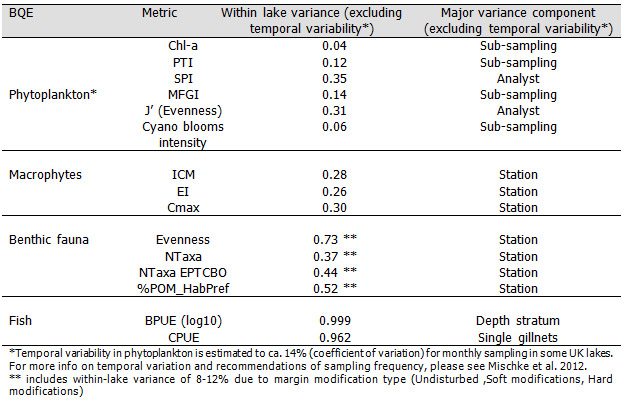 Table 2
Table 3. Minimum recommended sampling frequencies for three phytoplankton metrics in three GIGs. The number of months and years mean 1 sample taken for each of the number of months in each of the number of years. For example for NGIG, chlorophyll a should be sampled at least once in 2 different months in each of 3 different years or once in 3 different months in each of 2 different years, meaning 6 samples altogether.
| Central Baltic GIG | Mediterranean GIG | Northern GIG | |
|---|---|---|---|
| Chlorophyll a | 3 months for 4 years | 3 months for 3 years | 2 months for 3 years or 3 months for 2 years |
| PTI | 2 months for 4 years or 1 month for 6 years |
3 months for 3 years or 1 month for 6 years |
3 months for 3 years or 1 month for 6 years |
| Cyanobacteria | 1 month for 6 years | 1 month for 6 years | 1 month for 6 years |
Implication
Different BQEs and metrics require different monitoring and sampling designs based on the dominant sources of uncertainty.
For phytoplankton, the greatest source of variability is seasonal variability and analytical variability. The former can be reduced by utilising metrics based on repeated sampling during specific seasons (e.g. growth season or summer months) with higher frequency in eutrophic lakes, especially to catch harmful blooms. Minimum sampling frequency varies by metric and GIG, but should always cover the late summer period (Table 8). The analytical variability can be reduced by following standard counting guidance and consistent training within Member States and across Europe.
Macrophyte field method should be based on transects covering the whole depth zone and different littoral habitats. Sampling can be restricted to hydrophytes in lakes dominated by eutrophication pressure, whereas helophytes should be sampled if water level fluctuation or hydromorphological changes are assessed. More transects are needed at both ends of the trophic gradient to reduce uncertainty in status assessment.
Macroinvertebrate assessment of shoreline modifications should be based on composite or habitat specific sampling (depending on region) at various stations representing the whole range of morphological shore modification. The calculation of the whole-lake assessment score may be supported by conducting a physical habitat survey along the whole lake perimeter, relating this to the respective biological MMI, and then calculate a weighted average of site-specific MMI scores.
Fish assessment should be based on sampling of all depth strata with many gillnets. Hydroacoustic methods provide cost-effective assessment of fish abundance.
Further reading
Dudley B, Dunbar M, Penning E, Kolada A, Hellsten S, & Kanninen A. 2011. WISER Deliverable D3.2-2: Report on uncertainty in macrophyte metrics
Mischke, U., Stephen Thackeray, Michael Dunbar, Claire McDonald, Laurence Carvalho, Caridad de Hoyos, Marko Jarvinen, Christophe Laplace-Treyture, Giuseppe Morabito, Birger Skjelbred, Anne Lyche Solheim, Bill Brierley and Bernard Dudley 2012. Deliverable D3.1-4: Guidance document on sampling, analysis and counting standards for phytoplankton in lakes.
Thackeray S, Nõges P, Dunbar M, Dudley B, Skjelbred B, Morabito G, Carvalho L, Phillips G, Mischke U. 2011. WISER Deliverable D3.1-3: Uncertainty in Lake Phytoplankton Metrics, June 2011.
Winfield, I. J., Emmrich, M., Guillard, J., Mehner, T., Rustadbakken, A., 2011. Guidelines for standardisation of hydroacoustic methods. WISER deliverable 3.4-3.
06 Uncertainty levels associated with metric variability in multi-metric fish indices can be managed to increase the confidence in ecological status class assignment
Key message
Technical and monitoring design factors (gear, sampling season, and survey protocol including sampling effort), and natural and anthropogenic pressures all affect the variability of fish metrics. The within-system variability is notably larger than the between-system variability. This effect is probably due to natural factors and sampling bias and hence the standardization of sampling methods and more robust fish metrics will increase the robustness of the use of the BQE fish in transitional waters.
Evidence
Potential 'noise' factors (i.e. inherent variability) confounding biological quality metrics can be technical (i.e. those linked to the method of assessment including sampling effort) or natural (physicochemical and biological). We applied linear models using fish metrics as response variables and a suite of covariates to explain the metric scores and identify the sources of variability affecting them. The resulting best models contained from 3 to 14 covariates but explained only a relatively small amount of the total variance. With the available dataset, the best models explained less than 40 % of fish metric variability (with a maximum 22% for lagoons and 40% for estuaries). The remaining variability was mainly within-estuary or lagoon and can probably be attributed, at least in part, to both a habitat effect that was not accounted for in the models and to the influence of biological interactions in influencing community structure.
The effect of sampling effort on fish metrics could not be assessed in the previous analysis but this factor will have an important effect on the variability of fish metrics. The analysis showed that sampling effort is an important source of variability in fish metrics of the EFAI index, especially metrics dependent on number of species, which are common to several other fish-based indices (see figure below). In turn, metrics based on percentages (derived from the abundance of marine migrants, estuarine residents, piscivorous species) showed a lower sensitivity to the increase in sampling effort, with values stabilizing after a fewer hauls compared to metrics based on species richness. The stabilization of metrics based on species richness varied between salinity zones, with an increasing number of hauls generally required at higher salinities. In contrast, salinity zone did not have that effect on metrics presented as percentage abundance for different guilds.
The sensitivity of richness-based metrics is caused by including in the analysis species with an apparent abundance below a certain threshold, which prevent the complete characterisation of their presence. These rare species, in some cases a single individual collected on a single occasion, would only be incidentally recorded and therefore add random variability to diversity-based metrics. This in turn affects the relative scores and the outcomes of the assessment. A similar effort-related bias may be an issue for density-based metrics if fish distribution is very patchy (i.e. schooling fish or those aggregated in specific habitats) and insufficient replicates are taken to fully characterise the patchiness in their distribution. It is apparent that to overcome a potential large source of error, the reference conditions must be defined according to the level of effort used in the monitoring programme or, conversely, the monitoring must be carried out at the same level of effort used to derive the reference.
Improving accuracy without having to increase efforts may be possible by greater use of proportion metrics or the use of less-selective gear sets or multi-gear approaches. Alternatively, a more pragmatic decision could be made based on the probability of capture, thus considering in the analysis only those aspects for which the sampling method and level of effort allows for a reliable and quantitative estimation. Two possible options were identified: (1) weighting of metrics by precision or by species relevance, or (2) pooling samples to ensure sampling events provide greater habitat or temporal integration (i.e. larger effective samples).
Implication
A minimum effort is required to minimize misclassification (i.e. prevent wrong ES quality class assignment). A better, more robust assessment may be possible but residual variability should be accounted for and explained and cannot be decreased without increasing the number of replicates (effort). Reducing uncertainty in ES assessments will require a better knowledge of habitat partition within systems, understanding of metrics behaviour and precision, testing new combination rules allowing metric weighting by robustness and importantly research on new and more robust sampling tools and methods.
Further reading
Courrat A, Lepage M, Alvarez MC, Borja A, Cabral H, Elliott M, Franco A, Gamito R, Neto JM, Pérez-Domínguez R, Raykov V, Uriarte A (2012) The ecological status assessment of transitional waters: an uncertainty analysis for the most commonly used fish metrics in Europe. In: WISER Deliverable D4.4-2 (part 2)
Pérez-Domínguez R, Alvarez MC, Borja A, Cabral H, Courrat A, Elliott M, Fonseca V, Franco A, Gamito R, Garmendia JM, Lepage M, Muxika I, Neto JM, Pasquaud S, Raykov V, Uriarte A (2012) Precision and behaviour of fish-based ecological quality metrics in relation to natural and anthropogenic pressure gradients in European estuaries and lagoons. In: WISER Deliverable D4.4-5